Production RAG Architecture: Chunking, Embeddings, Hybrid Retrieval, and Anti-Hallucination. The Complete Guide
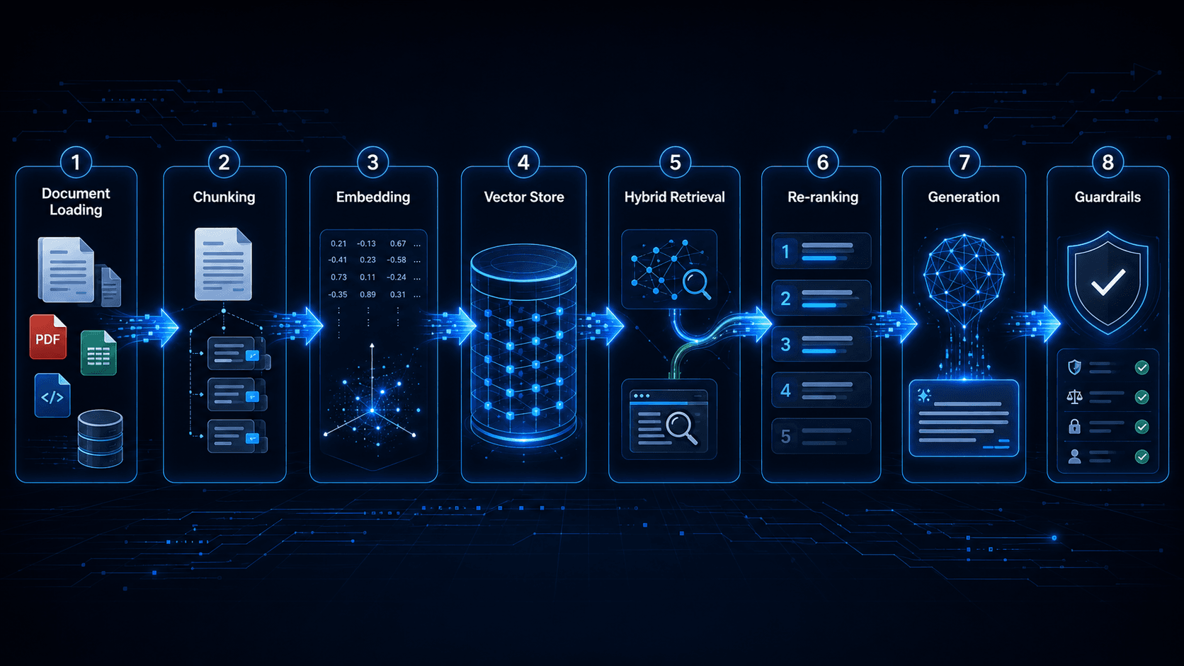
RAG is not a single thing. It is a pipeline with seven or eight discrete engineering decisions, each of which significantly affects accuracy. This is the complete architecture guide based on what we have learned shipping RAG systems to production.
Retrieval-Augmented Generation has become the standard architecture for LLM-based systems that need to answer from specific content rather than from the model's training data. The concept is straightforward: retrieve relevant content from your knowledge base, then pass that content to the LLM along with the user's question so it can answer from your actual information.
The implementation is not straightforward. There are seven or eight significant engineering decisions in a RAG pipeline, and getting even two or three of them wrong is enough to produce a system that returns confident, plausible-sounding wrong answers in production. This post covers each decision in detail, with the choices we have found work in practice.
The pipeline overview
A production RAG pipeline has two phases: indexing (offline, runs when your knowledge base content changes) and retrieval (online, runs on every user query).
The indexing pipeline:
- Load documents from source
- Clean and normalize content
- Chunk documents into retrievable segments
- Embed each chunk using an embedding model
- Store chunks and embeddings in a vector store
The retrieval pipeline:
- Receive user query
- Embed the query using the same embedding model
- Retrieve candidate chunks (vector similarity search plus optional BM25)
- Re-rank candidates
- Build the context window
- Generate the response
- Apply post-generation guardrails
Each step has decisions that compound. Let us go through them.
Document loading and preprocessing
The quality of your retrieval is bounded by the quality of your input documents. If your source content is poorly structured HTML, PDF with inconsistent formatting, or Word documents with complex layouts, your chunking quality will suffer regardless of how sophisticated your chunking strategy is.
Cleaning
Before chunking, remove content that does not contribute to retrieval quality:
- Navigation menus, headers, and footers from HTML documents
- Page numbers and running headers from PDF conversions
- Boilerplate text that appears in every document, such as "All rights reserved" or "Confidential"
- Repeated disclaimers or legal notices that should not match user queries
- Content in languages you are not indexing
Also normalize:
- Unicode characters, fancy quotes, dashes, and other typographic characters that differ between the source and how users type queries
- Whitespace, collapse multiple spaces, remove trailing whitespace, and normalize line endings
- Encoding artifacts from PDF extraction (the common case is ligatures being extracted as separate characters: "fi" becoming "f i")
Metadata extraction
Before chunking, extract document-level metadata that will be attached to every chunk from that document:
- Document title
- Author or source system
- Category or taxonomy tags
- Publication date or last-updated date
- Document ID for deduplication
This metadata enables filtered retrieval, restricting the search to chunks from documents published after a certain date, or tagged with a specific category, which significantly improves precision for many query types.
Chunking strategy
Chunking is the decision that most teams get wrong first. The naive approach, split every N characters, produces chunks that start and end mid-sentence, destroying the semantic coherence that makes retrieval work.
Sentence-aware chunking
The baseline we use is sentence-aware chunking: split at sentence boundaries, with a target chunk size and an overlap window. Our defaults:
- Target chunk size: 2,800 characters
- Overlap: 350 characters
- Hard boundary types: paragraph breaks, section headings, and document-defined sections
The overlap ensures that a concept that spans a chunk boundary is present in at least one complete chunk. Without overlap, a sentence like "The treatment protocol is described below. It consists of three phases." split at the period between those sentences would result in a chunk where "the treatment protocol" is described but the word "below" points to content that is in the next chunk. With overlap, the next chunk begins 350 characters before the end of the previous chunk, so that connective sentence is present in both.
Hierarchical chunking
For longer documents with clear section structures, such as technical documentation, clinical guidelines, and legal documents, hierarchical chunking works better than flat chunking. The document is first split into sections by heading level, then each section is split into chunks. Chunks inherit the section title as metadata, which provides context that would otherwise be lost.
A flat chunk that reads "The recommended dose is 10mg twice daily" is ambiguous without context. A hierarchically chunked version knows this chunk came from the section "Dosing for Adults with Renal Impairment", which makes retrieval and generation much more accurate for related queries.

Small-to-large chunking
An increasingly effective strategy for complex documents: index small chunks (300 to 500 characters, corresponding to a single idea or fact) for retrieval, but return the larger surrounding chunk (2,000 to 3,000 characters) to the LLM for generation. The small chunk is precise enough for accurate retrieval; the large chunk provides enough context for accurate generation.
This requires storing two representations of the same content: the small retrieval chunks linked to their parent large chunks. The overhead is worthwhile for knowledge bases where individual facts need to be retrieved with high precision.
Embedding models
The embedding model converts text into a dense vector representation. The similarity between two vectors corresponds to the semantic similarity between the texts. Every retrieval result depends on this mapping being accurate.
Model selection
The tradeoffs between embedding models come down to four factors: vector dimension (larger equals more expressive but more storage and compute), context window (how much text can be embedded at once), performance on your specific domain, and cost.
Our standard choice for production is text-embedding-3-large from OpenAI (3,072 dimensions). It performs well across a broad range of domains without domain-specific fine-tuning. For cost-sensitive applications where we can tolerate slightly lower recall, text-embedding-3-small (1,536 dimensions) is a reasonable tradeoff. For fully on-premises or open-source deployments, BAAI/bge-large-en-v1.5 is consistently strong on MTEB benchmarks.
We tested this on our RAG pipeline project for MyQRGuide. Switching from text-embedding-ada-002, the older OpenAI model with 1,536 dimensions, to text-embedding-3-large improved retrieval hit rate, meaning the relevant source appeared in the top 5 results, from 61% to 83% on a test set of 200 representative queries, which represents a 22-point improvement with no other changes to the pipeline.
Embedding consistency
The same model must be used for indexing and retrieval. This sounds obvious but causes real problems when you upgrade the embedding model. Existing embeddings in the vector store were created with model version A. New queries are embedded with model version B. The vectors are not compatible and retrieval quality collapses. Upgrading the embedding model requires re-indexing the entire knowledge base. Plan for this in your architecture: store the model version alongside each chunk's embedding, and build tooling to re-index when the model changes.
Vector storage
Your indexed chunks and their embeddings need to live somewhere that supports approximate nearest neighbor (ANN) search efficiently at your scale.
Options
The landscape of vector stores has expanded rapidly. The main options:
- Pinecone: Managed vector database, no infrastructure to run. Good ANN performance, generous free tier for development, and predictable pricing. Our default for new projects where operational simplicity is the priority.
- pgvector: PostgreSQL extension that adds vector similarity search. Good choice if you are already running PostgreSQL and want to keep your stack simple. ANN performance at scale for over 100k vectors requires HNSW indexing, which is available in pgvector but requires tuning.
- MySQL with vector columns: MySQL 9.0 added vector support. Viable for smaller knowledge bases under 50k chunks if you are already on MySQL. We used this for an early prototype because the operational cost of adding a separate vector store was not justified at that scale.
- Weaviate, Qdrant, Chroma: Purpose-built vector databases with more advanced filtering and multi-vector support. Worth considering for complex retrieval requirements.
Hybrid retrieval: vector plus BM25
Pure vector similarity search is good at finding semantically related content. It is less good at finding exact keyword matches, proper nouns, product names, codes, and other terms where the user knows the exact word and wants exact matches. A query for "ICD-10 code Z87.891" should return the exact code; vector search will return documents that are semantically related to smoking history, which is what that code means, but may rank the exact code match lower than it should.
BM25 is the classic TF-IDF-based ranking algorithm used by traditional search engines. It is excellent for exact keyword matching and poor at semantic understanding. Hybrid retrieval combines both:
- Run a vector similarity search → top N candidates
- Run a BM25 keyword search → top N candidates
- Merge the two result sets using Reciprocal Rank Fusion (RRF) or a weighted combination
- Re-rank the merged set
RRF is our default merging strategy because it is parameter-free and robust. The formula: for each document, sum 1 / (rank_in_list_1 + k) for each list it appears in, where k=60 is the standard value. Documents that appear in both lists with high ranks score very well. Documents that only appear in one list still contribute.
In our production RAG pipeline, hybrid retrieval improved recall at k=5 by roughly 15 percentage points compared to vector-only retrieval, with the largest gains on queries that included product names, codes, and technical terminology.

Re-ranking
The initial retrieval step optimizes for recall, returning a set of candidates that contains the relevant content. Re-ranking optimizes for precision, putting the most relevant content at the top of that set, so the LLM sees the best material first.
Cross-encoder re-rankers, models that take both the query and a candidate chunk as input and score relevance directly, consistently outperform bi-encoder similarity scores for re-ranking. Cohere Rerank and cross-encoder/ms-marco-MiniLM-L-6-v2 (open-source) are practical options. The tradeoff: cross-encoders are slower and more expensive than the initial retrieval step. We run them on a smaller candidate set (top 20 from hybrid retrieval, re-ranked to top 5 for generation).
The technique we use is Maximal Marginal Relevance (MMR) as a final step after re-ranking. MMR selects candidates that maximize relevance while penalizing redundancy; if two chunks say essentially the same thing, MMR will prefer one of them plus a different relevant chunk over both saying the same thing. This prevents the LLM's context window from being filled with redundant content.
Context window construction
After retrieval and re-ranking, you have your top-k chunks. How you present them to the LLM matters.
Context ordering
LLMs have a recency bias and a primacy effect; they attend more strongly to content at the beginning and end of the context window than to content in the middle. Put the most relevant chunk first or last, not buried in the middle of five chunks.
Metadata in context
Include document metadata in the context prompt. The source document title, date, and author give the LLM context about the provenance of the information, which improves citation accuracy and helps it weight more recent sources appropriately.
Context length
More context is not always better. A larger context window increases the risk of the LLM being distracted by marginally relevant content. We typically pass 3 to 5 chunks, roughly 8,000 to 15,000 tokens, rather than the maximum context length, and measure accuracy on a test set at different context lengths to find the optimal for our specific knowledge base.
Confidence thresholding and fallback
Not every user query can or should be answered from the knowledge base. A query that does not match anything in the knowledge base should not result in a hallucinated answer; it should result in an honest "I don't know" or a redirect to a human.
Confidence threshold
We implement a confidence threshold based on the similarity score of the top retrieved chunk. If the best match has a cosine similarity below a threshold, we use 0.45 as the default calibrated on a representative test set, we consider the query out-of-scope and return a fallback response rather than generating from low-confidence context.
The 0.45 threshold was established by plotting the distribution of top-chunk similarity scores for in-scope and out-of-scope queries on our test set and finding the score that minimized false positives (answering out-of-scope queries) and false negatives (refusing to answer in-scope queries). This calibration step is specific to each knowledge base and should be redone whenever the knowledge base content changes significantly.
Fallback responses
A fallback response should acknowledge the limitation honestly and provide a useful alternative: "I don't have information about that in my knowledge base. Here is how to reach a human who can help." Hallucinating an answer is never the right fallback.
In our production system, the fallback rate started at around 28% when the knowledge base was first deployed due to many queries not being covered by initial content. After six weeks of monitoring failed queries and adding content to cover the most common gaps, the fallback rate dropped to 12%. Monitoring what your system does not know is as important as monitoring what it does know.
Post-generation guardrails
Even with a well-built retrieval pipeline, LLMs can generate content that is not supported by the retrieved context, particularly when the query asks for something that is not directly stated but the model can "reason" from adjacent content. Post-generation guardrails check the generated response against the retrieved context.
Groundedness check
After generation, a separate model call or a dedicated groundedness classifier evaluates whether each factual claim in the response is supported by the retrieved context. Claims that are not supported by the context are flagged for removal or human review.
This step adds latency and cost. We use a lightweight classifier rather than another GPT-4 call for the groundedness check to keep the overhead manageable, adding a few hundred milliseconds rather than a full generation cycle.
Citation enforcement
Requiring the LLM to cite the specific source chunk for each factual claim in the response serves two purposes: it makes hallucinations visible (a claim with no citation is a red flag), and it provides users with provenance information they can verify. We instruct the LLM to cite sources in the format [Source: document_title, section] and then validate that cited sources actually appear in the retrieved context.
Monitoring in production
A RAG system that was accurate at launch will drift as your knowledge base content changes, the distribution of user queries shifts, or the underlying model changes. Production monitoring should track:
- Fallback rate (queries below confidence threshold)
- User feedback signals (such as thumbs up or down and follow-up clarification questions)
- Retrieval hit rate on a fixed test set, run weekly
- P95 latency by pipeline stage, including retrieval, re-ranking, and generation
- Groundedness check failure rate
When the fallback rate increases, it usually means users are asking about topics not in the knowledge base, so you must add content. When the retrieval hit rate decreases, it usually means either the knowledge base has changed in a way that breaks existing retrieval patterns or the query distribution has shifted, so you must review the test set and re-calibrate the pipeline.
RAG done well is a significant engineering investment. The architecture described here reflects what we have learned from building and iterating on production systems. If you are planning a RAG implementation for a healthcare knowledge base, a product documentation assistant, or a domain-specific Q&A system, we can help you avoid the mistakes we made so you start with a foundation that holds up in production.
Related service
AI Development & Automation
Production RAG pipelines, LLM integrations, and AI workflow automation for healthcare and e-commerce.
Written by
Founder & CEO
Gaurang Ghinaiya is the Founder & CEO of Nexios Technologies. He is passionate about building innovative software solutions that drive business growth. With years of experience in technology leadership, he guides teams toward excellence.